
Version 4.1.6.2
Standard Filter
You can set a Standard Filter from within the AutoFilter drop-down, or you can go there through the Data menu by selecting Data–>Filter–>Standard Filter. Now let’s look at the question we ended the last tutorial with: How many females over the age 40 had a case in 1978. We saw we could get this by manually putting checkmarks in every age that was greater than 40 using AutoFilter, but how do we do this using Standard Filter?
If you had already filtered for 1978 and for Female using AutoFilter, you could go to the drop-down for any of the columns and select Standard Filter. You would get this window:
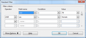
Standard Filter window
You will see that the filters you already have in place are reflected in this window. For the first filter it says that the field name of “year” with a condition of “=” and a value of “78” has been selected. Going to line 2, we see one big thing already, which is that there is an operator, and in this case the operator is “AND”. It goes on to say Field name of “sex”. condition of “=”, and value of “female”. But that Operator area is important, since you can also select OR as an operator. This is one of those things that you cannot do using AutoFilter. If we selected OR as an operator here, it mean that we would select any case that occurred in 1978, or any case that occurred involving a female. But we could have cases that involved females that occurred in other years, or we could have cases in 1978 that involved males. The general rule to remember is that using AND reduces the size of your results, and using OR increases the size.
So, to get the answer we are looking for we need to add one more filter here. So on line 3, select “AND” as the operator, “age” as the Field name, “>” as the Condition, and “40” as the value. Though there is a drop-down for Value, you are better off just typing in 40 here. The drop-down just shows every value already existing in the age field, and you may not have the exact number you want in there. When you are done, click OK and you will see the six cases we noted previously.
Another great advantage of using the Standard Filter is the increased flexibility of the Condition criterion. Using AutoFilter, every filter is implicitly set to Equal as the condition. But the Standard Filter gives you a ton of options:
- =
- <
- >
- <=
- >=
- Largest
- Smallest
- Largest %
- Smallest %
- Contains
- Does not contain
- Begins with
- Does not begin with
- Ends with
- Does not end with
The first few are pretty clear. Equals, less than, greater than, less than or equal, and greater than or equal are all pretty standard conditions. Largest is like the Top 10 we saw in AutoFilter, but you can specify a number other than 10, such the 5 largest values in the field. And the opposite, smallest, is also available for when you need to go in the other direction. Largest % and Smallest % let you get the top 1%, for instance, or the bottom as the case may be. The remaining options are perhaps best thought of as string operations. Here are some examples:
- For the Field name select Sex, condition is “Contains”, and type in value “em”. In this case, it is equivalent to selecting on “equals female”.
- For the Field name select Race, condition is “Does not contain”, and type in value “bl”. This will have effect of filtering out everyone in the dataset who is black.
- For the Field name select Sex, condition is “Begins with”, and type in value “m”. This will be equivalent to selecting “equals male”.
- For the Field name select Sex, condition is “Does not begin with”, and type in value “f”. This will also be equivalent to selecting “equals male”.
I’m sure you can work out using Ends with and Does not end with from these examples.
You can combine filters in other ways. For instance, suppose you wanted to select everyone in the dataset who is 21 years of age or older, but not older than 65. You would do this with two filters using Standard Filter. For the first one, Field name is Age, condition is “greater than or equal”, and type in value “21”. Then for the second filter, Field name is Age, condition is “less than or equal”, and type in “65”. Click OK, and you have your answer.
And you can do the opposite type of filter using the OR operator. To get everyone who is either younger than 21 or older than 65, make the first filter “age”, “less than”, and “21”, then for the second filter use “OR”, “age” “greater than”, and “65”. This will give you the group that was excluded in the previous filtering.
And there is more. If you look at the lower left of the Standard Filter window you see More options. Clicking this opens a bottom section to the window. Here you can make selections like:
- Case sensitive – Useful if you need to distinguish strings which might have lower case and upper case and you need to select on that basis.
- Range contains column labels – This should be checked by default. Usually the first row contains the labels for each field, and you wouldn’t want them mixed up in the filtering.
- Regular expression – This allows you to use regular expressions in any filter which is set to either “Equal” or “Not equal”. In particular this is how you would use wildcards in your filter. For a list of regular expressions supported in Calc go here.
- No duplication – This will not show two rows that are identical, only one of them.
- Copy results to – A very interesting option, this lets you apply a filter, then copy the resulting data to a new location. For example, create new sheet and give it a name, such as “copied Results from Filter. Then set up a filter. In my sample spreadsheet I took the filter that selected people under 21 or over 65. I clicked “Copy results to…” and then clicked on the roll-up icon on the far right of that row. I went to my new sheet, clicked on cell A1 of that sheet, then clicked the roll-down icon to return to my window, then clicked OK. All of my results got copied to the new sheet. One interesting change is that everything renumbered.
Advanced Filters
This is in some ways simpler than you might think. The idea here is to do everything in the spreadsheet itself. You enter your criteria in cells of the spreadsheet. So I created a new sheet to do a filter using the AND operator, and copied it from the reduced dataset sheet. Advanced filtering always assumes you are operating on the data in the current page. I moved over to columns I through N, selected the six cells on Row 1 for those columns, then clicked Merge and Center. Then I typed in “AND Filter”, made it bold, 12-point, and added a blue background. Under that I copied my six column headers from my dataset in Row 2. In row 3 I can add the criteria I am looking for in my filter. If I am using Equals I can just enter value (equals is assumed, in other words), but if I want to do anything using inequalities I need to type that in. So in this row I type 78 under the Year field, >40 in the Age field, and male in the Sex field. Once I have done this, I can go to Data–>Filter–>Advanced Filter. You will see this window:

Advanced Filter window
First, highlight the range of cells that contain the data you want filtered. For my set, it is cells A1 through F582. Then go to Data–>Filter–>Advanced filter, and select the range of cells that have the column labels and the criteria, which for my example is cells I2 through N3. I click the roll-up icon to the right of the range field, then click-and-drag to select this range, and then click the roll-down icon. Click OK and I get the result. What this will do is hide every row that does not meet these criteria. In my example, that results in 7 rows, or 7 cases selected.
When doing an AND filter, putting the criteria on the same row will produce the results you want. To get an OR filter, put them on different lines. To replicate the one I did previously, I set up a sheet with the data, created a filter section like I did above, but in this case I entered <21 in cell L3 (L is the column for Age in my filter criteria), and >65 in cell L4. This will select everyone in the dataset who is under 21 or over 65. Execute the filter like the above example. In my example that resulted in 395 cases selected.
Standard vs. Advanced
You can do many of the same things using these two methods, but I find that “Advanced” is a misleading name. To me, the Standard method is more flexible and easy to work with. The one advantage to Advanced that I can see is that you can have all of the filter criteria readily visible on the same sheet as the data, and I can see that being handy. Still, if I only had time to master one approach, I would master Standard Filters.
The sample spreadsheet used in this tutorial can be downloaded from here.
Listen to the audio version of this post on Hacker Public Radio!
 Save as PDF
